Basics

Time-varying AR(p) [autoregressive] models provide a model-based approach for estimating time-dependent return rates in time series, which can act as an early warning of a critical transition. In time-invariant AR(p) models, the inverse of the characteristic root, λ, of a fitted AR(p) model is similar in magnitude to the dominant eigenvalue of the Jacobian matrix computed at a stationary point of a deterministic discrete-time model. Values of λ near zero imply that the state variable returns rapidly towards the mean; this central tendency diminishes as values approach one.

Time-varying AR(p) models assume that the coefficients of the AR(p) model can change through time, thereby allowing estimation of the time-dependent characteristic root as it varies along a time series up to a transition. To the general form of time-varying AR(p) models we can incorporate measurement error to construct a state-space model that can be fit using a Kalman filter. Fitting with a Kalman filter gives maximum likelihood parameter estimates, and likelihood ratio tests (LRT) can be used for statistical inference about the parameter estimates, such as Akaike’s Information Criterion (AIC) for model selection.

Example

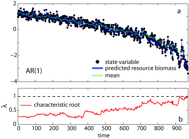
We fitted time-varying AR(p) models with p = 1, 2, and 3 to the time series after log-transforming and standardizing the data. For all cases, we computed time-varying AR(p) models for which only the mean was allowed to vary through time and compared them to AR(p) models for which both the mean and the autoregressive coefficients were allowed to vary with time. The log-likelihood ratio test (LRT) indicated that the models with varying autoregressive coefficients were significantly better than the mean-varying-only models. Comparing across models, the best fit was derived with the time-varying AR(1) model (panel a). We computed the inverse of the characteristic root λ of time-varying AR(1) models at each point in the time series from the estimates of their autoregressive coefficients (panel ). Values of λ approaching 1 imply critical slowing down, while values of λ > 1 imply loss of stationarity. We found a clear increasing trend in λ (τ = 0.736) in the time-varying AR(1) model (panel ), as the time series approached the transition.